Model of GTA evolution by infectious transfer

Here's the description of my model addressing Explanation 1 for GTA persistence.  For now I've just pasted in the text of a Word file I prepared about 10 days ago.

A constant-population-size model of large-head GTA transmission

(Based on Xin Chen’s model, but with stepwise generations and without logistic growth.)

Assumptions:

The population:

1.     Population size is constant.  Loss of GTA+ cells due to lysis during GTA production is made up by growth of all cells after the transduction step.

2.     Dense, well-mixed culture in liquid medium (so cells frequently encounter GTA particles)

GTA production:

3.     GTA particles come in two sizes.  Small particles contain 4 kb DNA fragments.  The hypothetical large particles contain fragments that must be at least 14 kb (the size of the GTA gene cluster) but could be as big as 50 kb. 

4.     The number of GTA particles a cell produces does not depend on the proportion of small and large particles.

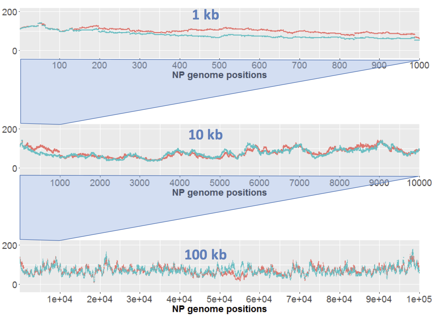
5.     DNA packaging by GTA is random; all parts of the cell’s genome are equally represented.  But in this model we only consider the particles containing the full-length GTA cluster.

6.     This is the killer:  If the cell’s chromosome is 5 MB and the large-particle capacity is 15 kb, only 2x10^-4 of large particles will contain complete GTA gene clusters (will be G+ particles).  If we change the large-particle capacity to 20 kb, then about 1x10^-3 of large particles will contain a complete cluster.  A 50 kb capacity and a 3 MB chromosome would probably get it up to about 10^-2.  (And this ignores the recombination machinery’s need for homologous DNA flanking the GTA cluster to promote recombination.)

Transduction:

7.     GTA- cells completely lack the main GTA gene cluster.  They can only be converted to GTA+ by homologous recombination with GTA-containing DNA from G+ particles.

8.     GTA particles cannot tell the difference between GTA+ and GTA- recipients.  Particles capable of transducing GTA- cells to GTA+ can also ‘transduce’ GTA+ cells to GTA+.

9.     All GTA particles produced in one cycle are taken up by and transduce cells in that cycle.  (The efficiency of infection and recombination is 1.) 

10.  The model ignores large and small GTA particles that don’t transduce GTA+.

11.  Each cell takes up only one G+ particle (or none).  This is reasonable, since the number of G+ particles is always going to be much smaller than the number of cells.

Parameters:

F    Initial frequency of GTA+ cells (we want to consider a wide range)

c    Fraction of GTA+ cells producing GTA particles (and consequently lysing).  (In wildtype lab cultures this is <3 o:p="">

b    Number of GTA particles produced by each burst.  Default value is 100.  (We have no actual measurements.)

µ    Fraction of GTA particles that are large.  (We expect this fraction to be small, since large particles have not been observed.)

T    Fraction of large GTA particles that are G+ particles (able to transduce GTA).  (This is limited by genome size, GTA gene cluster size, and the DNA capacity of these hypothetical particles.  Plausible values are between 10^-2 and 10^-4.)

G   µ * T Fraction of GTA particles that contain complete GTA genes.

What happens in one generation:

GTA production and cell lysis:

N   Proportion of GTA particles to cells remaining in the medium after GTA+ cells have burst. 

      = (Fcb)/(1 – Fc)  (Note: Fcb is the GTA production per original cell.  1 – Fc normalizes this to the number of cells remaining after lysis.)

N⁺  Proportion of GTA particles, per remaining cell, that carry the complete GTA gene cluster (are ‘G+’ particles able to transduce the GTA-production genotype to GTA- cells). 

= NµT   =  NG

Fraction of surviving GTA+ cells per original cell (will be normalized to remaining cells later): = F(1 – c)

Transduction:

Fraction of GTA- cells transduced to GTA+: N⁺(1 – F).  {Note: the 1 – F corrects for the G+ particles that attach to and ‘transduce’ GTA+ cells.) 

Fraction of GTA+ cells (per original cell) after transduction:  F(1 – c) + N⁺(1 – F).  (Note: F(1 – c) removes cells killed by lysis, N⁺(1 – F) adds cells gained by transduction.)

Fraction of GTA- cells (per original cell) remaining after transduction:  (1 – F) – N⁺(1 – F).  (Note: 1 – F is the original fraction of GTA- cells, N⁺(1 – F) removes cells lost by transduction to GTA+.)

Cell growth:

Now we normalize the cell numbers to ‘per remaining cell’:

Total fraction of cells remaining after GTA production and transduction:

            1 – (Fc)  (Note: To normalize, divide the above cell fractions by this value.)

Fraction of GTA+ cells after one complete cycle:

F’ = F(1 – c) + N⁺(1 – F) / 1 – Fc

How to evaluate the change in the proportion of GTA+ cells?

We can expand N⁺ and pull out the F, then look at the before/after ratio:

F’   = F * (1 – c) + c * b * F * µ * T * (1 – F) / 1 – (F * c)

      = F * ((1 – c) + C * b * µ * T * (1 – F) / 1 – (F * c)

F’ / F = (1 – c) + c * b * µ * T * (1 – F) / 1 – (F * c)

When the value of this expression is greater than 1, GTA+ is increasing; when it is less than 1, GTA+ is decreasing.

For simplicity, below I combine b, µ & T as the compound variable W.

What happens if we vary F, holding everything else constant?

Increase of GTA+ depends only on W.  If W is >1, GTA+ increases.  If W is <1 decreases.="" gta="" o:p="">

The rate of change is very slow when F is close to 1 (when almost all cells are GTA+), and fast when F is close to 0 (when almost all cells are GTA-).

What happens if we vary c, holding everything else constant?

C affects how fast change happens, but not its direction.  If W>1, GTA+ still spreads; if W<1 decreases="" gta="" o:p="" still="">

What happens if we vary W, holding everything else constant?

If W<1 always="" be="" denominator.="" numerator="" o:p="" smaller="" than="" the="" will="">

If W>1, the numerator will always be smaller than the denominator.

In both cases., all the other parameters cancel out.  This confirms that the direction of selection o GTA+ depends only on whether W is higher or lower than 1.

Would the result change if the population were growing?

I don’t think so, since GTA+ and GTA- cells grow at the same rate.

Since plausible values of W are all much lower than 1, I conclude that GTA+ cells cannot increase by GTA-mediated transduction of GTA- cells to GTA+.

GTA could spread by transduction if it did preferentially package the GTA gene cluster into its particles.  Of course, then it would be a phage.

How the model’s assumptions affect this outcome:

Basically, all the assumptions are either neutral or increase the chance that GTA+ will spread. Making the simulation more realistic would just make things worse for GTA+, not better.

The population:

1.  Population size is constant.  Loss of GTA+ cells due to lysis during GTA production is made up by growth of all cells after the transduction step.

I don’t think adding growth would affect the outcome.

2.  Dense, well-mixed culture in liquid medium (so cells frequently encounter GTA particles).

If the culture were more dilute or poorly mixed, some GTA particles would not find new cells to attach to.  This would reduce the amount of transduction (effectively reducing W).

GTA production:

3.  GTA particles come in two sizes.  Small particles contain 4 kb DNA fragments.  The hypothetical large particles contain fragments that must be at least 14 kb (the size of the GTA gene cluster) but could be as big as 50 kb. 

This is the central assumption of the model.  The size of the small particles is known.  The hypothesized large particles could be as small as 15 kb (allows a bit of homologous sequence on each side of the cluster to promote recombination).  Phage capsids can in principle be very large, but it’s parsimonious to assume a modest size.

4.  The number of GTA particles a cell produces does not depend on the proportion of small and large particles.

Large capsids will require more capsid protein molecules.

5.  DNA packaging by GTA is random; all parts of the cell’s genome are equally represented.  But in this model we only consider the particles containing the full-length GTA cluster.

Experimental results show slightly less packaging of GTA sequences.  If this applies to the hypothetical large particles it would reduce production of G+ particles.  If particles preferentially package GTA, GTA would be a phage.

6.  This is the killer:  If the cell’s chromosome is 5 MB and the large-particle capacity is 15 kb, only 2x10^-4 of large particles will contain complete GTA gene clusters (will be G+ particles).  If we change the large-particle capacity to 20 kb, then about 1x10^-3 of large particles will contain a complete cluster.  A 50 kb capacity and a 3 MB chromosome would probably get it up to about 10^-2.  (And this ignores the recombination machinery’s need for homologous DNA flanking the GTA cluster to promote recombination.)

See point 3 above.

Transduction:

7.  GTA- cells completely lack the main GTA gene cluster.  They can only be converted to GTA+ by G+ particles.

Transduction depends on homologous recombination.  Small GTA particles can transduce functional alleles of individual GTA genes, replacing versions that became mutated or even deleted in an ancestor of the recipient cell.  But they cannot introduce GTA genes into cells that completely lack the GTA cluster, because there will be no homologous sequences to recombine with.

8.  GTA particles cannot tell the difference between GTA+ and GTA- recipients.  Particles capable of transducing GTA- cells to GTA+ can also ‘transduce’ GTA+ cells to GTA+.

I think some phages and conjugative plasmids may be able to detect whether potential hosts/recipients already have the element, but we have no evidence that transduction frequencies differ between GTA+ and GTA- recipients.  Wall et al (1975) surveyed 33 strains and found wide variation in both GA production and transduction, but no correlation between these abilities.

9.  All GTA particles produced in one cycle are taken up by and transduce cells in that cycle.  (The efficiency of infection and recombination is 1.) 

This is unlikely to be true, but assuming this increases the chance that each G+ particle successfully transduces a GTA- cell to GTA+.

If we were to relax this assumption the model would need to include an explicit uptake process and to specify what happens to particles that are not taken up.

10. The model ignores large and small GTA particles that don’t transduce GTA+. 

This should be OK, since these should not interfere with transduction by G+ particles, especially because their total number per cell will be small. Removing this assumption would make GTA + spread less likely.

11. Each cell takes up only one G+ particle (or none). 

This is a reasonable assumption, since the number of G+ particles is always going to be much smaller than the number of cells.  If the number of G+ particles were high, sometimes two G+ particles might inject their DNAs into the same s=cell, which would reduce the efficiency of transduction.

-->

Thinking about Gene Transfer Agent

I'm at Dartmouth for three months, working with Olga Zhaxybayeva's group to improve our evolutionary understanding of Gene Transfer Agent.  I'm writing an R-script simulation of the genetic exchange it causes (finally learning R), but my control runs with epistasis don't give the expected results.  So I'm writing this post and creating a Powerpoint deck to clarify my thinking.

First, what's Gene Transfer Agent?  A number of different kinds of bacteria produce 'transducing particles' called Gene Transfer Agents.  These look line small phage capsids but they don't usually contain phage DNA; instead they contain random fragments of chromosomal DNA.  In the best-characterized GTA ('RcGTA'), these are all 4.4 kb in length, which appears to be the DNA capacity of the tiny GTA heads.  Like phage, GTA particles inject their DNA into recipient cells (usually of the same species), where it often recombines with the chromosome and can change the cell's genotype.

GTA particles aren't infectious like phages are, both because they don't preferentially package the DNA that encodes them and because their heads are too small to contain this DNA.  The RcGTA head and tail proteins are encoded by a 14 kb gene cluster.  The sequences and organization of these genes strongly resemble that of homologous phage genes, so the known GTA systems are generally thought to have descended from what were integrated prophages. 

In lab cultures of cells with the RcGTA genes (Rhodobacter capsulatus cells), GTA is produced mainly after exponential growth has ceased, and only produced by a small subset of cells. Like release of phage particles from infected cells, release of GTA requires lysis of the cell, and the genes for the holin and endolysin proteins are encoded separately from the main RcGTA cluster.

There are good reasons to think that GTAs are not simply defective prophages that still can package small DNA fragments:

1. The main RcGTA gene cluster has been somewhat stably inherited over a very long time, maybe a more than a billion years.  Some descendants have lost all the genes, but about 25% of the 225 alpha-proteobacterial genomes examined have retained versions of a single large cluster, typically containing 14-17 co-transcribed genes, most of which encode capsid head and tail proteins.
2. Expression of this gene cluster is at least partly controlled by cellular regulatory mechanisms.  
3. Other genes, at other chromosomal locations, are also needed for efficient RcGTA production.

I just crunched some numbers from a detailed phylogenetic tree for the alpha-proteobacteria showing which taxa have GTA.  The large GTA cluster is only found in a subclade (148 taxa, 109 distinct species names); the authors estimate that this subclade is 1.0 - 1.4 billion years old.  57% of the taxa in this subclade have the large GTA gene cluster.

My goal for these three months is to generate models of GTA evolution (probably computer simulations) that evaluate the following candidate explanations for its persistence:

1. Infectious spread of GTA by rare large-head particles that package the 14 kb gene cluster.
2. Restoration of mutated GTA genes by unidirectional recombination with functional alleles from GTA-producing cells.
3. Beneficial recombination of chromosomal genes.

Flawed model for Explanation 1:  Nobody has seen the large heads postulated by Explanation 1, but nobody has explicitly looked for them.  The Zhaxybayeva lab already has an unpublished mathematical model that addresses this exp lanati on, created by a mathematically-inclined former post-doc.  It asks how frequent such heads would need to be in order to maintain GTA-producing cells in a mixed population of GTA+ cells and GTA- cells lacking the gene cluster.  The model assumes that  large heads are produced at frequency µ, and that these inject the GTA gene cluster into GTA- cells, converting them into GTA+ cells.  Only a small fraction of GTA+ cells are activated to produce GTA in any one generation, and these lyse after GTA production.  

The conclusion from this model is that GTA+ cells can persist at high frequency even if they only make large particle for every 10^5 normal small particles.  Because the model assumed a reasonable 'burst size' of 100 GTA particles per producer cell, this means that GTA+ can persist if only one cell in a thousand produces a single large particle.    

But I didn't think this result could be correct.  Since each cell lysis destroys a GTA+ cell and only one in a thousand creates a new GTA+ cell from a GTA- cell, the GTA+ population should be continually decreasing.  Production of new GTA+ cells only compensates for 0.1% of the loss of GTA+ cells.  

I initially had a hard time fully understanding the mathematics of this model.  It included expressions for logistic growth, which complicated the math without adding anything to its utility.  So I created my own version of this model, which gave a very different answer.

New model for Explanation 1:  I'm going to put the description of this model into another post, because here I want to get on to my beneficial recombination model.  Bottom line: the model's result is that transduction of the GTA gene cluster by large-head GTA particles can't come close to maintaining GTA+ cells in a mixed population even if every cell produces a large-head particle.  This is because:

1. All cells that produce GTA die; 
2. Only a small fraction of large-head particles will contain a complete gene cluster (maybe 0.1 to 1%); 
3. Except when GTA+ cells are rare, many particles will attach to GTA+ cells rather than to GTA- cells; 
4. In a natural environment many GTA particles will fail to find recipients.  (This issue isn't part of the model.)
5. To overcome these obstacles each GTA-producing cell would need to produce more than 1000 (10,000? 100,000?) large-head particles.

Finding the flaw in the lab's model:  Assuming that I understand the lab's model correctly, the main error is that it 'corrects' for the probability that a GTA particle will attach to a GTA+ cell rather than a GTA0- cell by multiplying by the number of GTA- cells rather than by their frequency.  Since the model assumes populations of 10^7 to 10^9 cells, this overestimates the amount of transduction by orders of magnitude, leading to a comparable underestimate of the frequency of large heads needed to maintain GTA+.

Model for Explanation 2:  I modified the basic structure of my Explanation 1 model to consider a related hypothesis.  Defective alleles of GTA genes are expected to arise by random mutation.  At least some of these will also prevent the cell from lysing when GTA production is induced.  These cells can still receive functional alleles of their defective genes from GTA particles produced by 'wildtype' cells, but they can't transmit their defective alleles to the wildtype cells because they can't produce GTA.  This asymmetry favours spread of functional alleles, and might be able to maintain GTA, although it wouldn't allow GTA+ to spread to cells that completely lack the GTA genes.

Like the model for Explanation 1, the result is a strong NO.  Because the models are very similar, it's not surprising (in retrospect) that spread of functional alleles faces the same obstacles

1. All cells that produce GTA die; 
2. Only a small fraction (about 0.1%) of particles will contain whatever GTA gene is mutated in a recipient cell; 
3. Except when GTA+ cells are rare, many particles will attach to cells with the functional allele rather than to those with mutated allele; 
4. In a natural environment many GTA particles will fail to find recipients.  (This issue isn't part of the model.)
5. To overcome these obstacles each GTA-producing cell would need to produce more than 1000 (10,000? 100,000?) large-head particles.

Models for Explanation 3:  Most microbiologists assume that GTAs are maintained in their genomes by selection for presumed benefits of chromosomal recombination.   They implicitly assume that randomizing the combinations of chromosomal alleles in a population creates a benefit strong enough to overcome the cost of the cell death associated with GTA production.  They don't explicitly assume this, because they're not used to thinking rigorously about evolutionary processes.  Instead their explanation usually relies on GTA-mediated recombination creating some specific beneficial new combination, and ignores the selective costs associated with other combinations.

In fact, many very smart people have spent many years looking for conditions where random chromosomal recombination creates benefits strong enough to maintain the genes that cause it.  These 'evolution of sex' models have identified some conditions, but usually these benefits are small and occur only under special circumstances.  Most of the time recombination appears to be a waste of time at best.

Recombination Model 1:  Way back when I was a new post-doc spending a year in Dick Lewontin's lab, I developed a computer-simulation model of recombination by natural transformation (Redfield 1988, Evolution of bacterrial transformaiton: Is sex with dead cells ever better than no sex at all?).  In this model I applied a relatively simple model of the evolution of sex to a population of naturally competent bacteria.  My first goal for addressing Explanation 3 is to adapt this model so it applies to recombination caused b GTA rather than by natural transformation.  I'll describe my progress (and current deadlock) in the next post.

Recombination Model 2:  Model 1 is 'deterministic'; it ignores random ('stochastic') events, effectively assuming that the population is infinitely large.  But the strongest benefits of recombination are now thought to arise from precisely the stochastic effects Model 1 ignores.  So I also want to make a stochastic model that tracks individual cells, or at least a model that takes stochastic processes into account.  I haven't started writing this model yet, but I might pattern it on the transformation model described by Takeuchi et al, 2014.

What's noise, what's Illumina bias, and what's signal?

The PhD student and I are trying to pin down the sources of variation in our sequencing coverage. It's critical that we understand this, because position-specific differences in coverage are how we are measuring differences in DNA uptake by competent bacteria.

Tl;dr:  We see extensive and unexpected short-scale variation in coverage levels in both RNA-seq and DNA-based sequencing. Can anyone point us to resources that might explain this?

I'm going to start not with our DNA-uptake data but with some H. influenzae RNA-seq data.  Each of the two graphs below shows the RNA-seq coverage and ordinary seq coverage of a 3 or 4 kb transcriptionally active segment.

Each coloured line shows the mean RNA-seq coverage for 2 or 3 biological replicates of a particular strain.  The drab-green line is from the parental strain KW20 and the other two are from competence mutants.  Since these genes are not competence genes the three strains have very similar expression levels.  The replicates are not all from the same day, and were not all sequenced in the same batch.  The coloured shading shows the standard errors for each strain.

We were surprised by the degree of variation in coverage across each segment, and by the very strong agreement between replicates and between strains.  Since each segment is from within an operon, its RNA-seq coverage arises from transcripts that all began at the same promoter (to the right of the segment shown).  Yet the coverage varies dramatically.  This variation can't be due to chance differences in the locations and endpoints of reads, since it's mirrored between replicates and between strains.  So our initial conclusion was that it must be due to Illumina sequencing biases.  

But now consider the black-line graphs inset below the RNA-seq lines.  These are the normalized coverages produced by Illumina sequencing of genomic DNA from the same parental strain KW20. Here there's no sign of the dramatic variation seen in the RNA-seq data.  So the RNA-seq variation must not be due to biases in the Illumina sequencing.

Ignore the next line - it's a formatting bug that I can't delete.

<200 and="" from="" in="" lower="" nbsp="" p="" segment.="" segment="" the="" to="" upper="">

How else could the RNA-seq variation arise? 

• Sequence-specific biases in RNA degradation during RNA isolation?    If this were the cause I'd expect to see much more replicate-to-replicate variation, since our bulk measurements saw substantial variation in the integrity of the RNA preps.
• Biases in reverse transcriptase?  
• Biases at the library construction steps?  I think these should be the same in the genomic-DNA sequencing.

Now on to the control sequencing from our big DNA-uptake experiment.

In this experiment the PhD student mixed naturally competent cells with chromosomal DNA, and then recovered and sequenced the DNA that had been taken up.  He sequenced three replicates with each of four different DNA preparations; 'large-' and 'short-' fragment preps from each of two different H. influenzae strains ('NP' and 'GG').  As controls he sequenced each of the four input samples.  He then compared the mean sequencing coverage at each position in the genome to its coverage in the input DNA sample.

Here I just want to consider results of sequencing the control samples.  We only have one replicate of each sample, but the 'large' (orange) and 'short' (blue) samples effectively serve as replicates.  Here's the results for DNA from strain NP.  Each strain's coverage has been normalized as reads per million mapped reads (long: 2.7e6 reads; short: 4.7e6 reads).

The top panel shows coverage of a 1 kb segment of the NP genome.  Coverage is fairly even over this interval, and fairly similar between the two samples.  Note how similar the small-scale variation is; at most positions the orange and blue samples go up and down roughly in unison.  I presume that this variation is due to minor biases in the Illumina sequencing.

The middle panel is a 10 kb segment.  The variation looks sharper only because the scale is compressed, but again the two traces are roughly mirroring each other,

The lower panel is a 100 kb segment.  Again the variation looks sharper, and the traces roughly mirror each other.  Overall the coverage is consistent, not varying more than two-fold.

Now here's the corresponding analysis of variation in the GG control samples.   In the 1 kb plot the very-small-scale position-to-position variation  is similar to that of NP and is mirrored by both samples.  But the blue line also has larger scale variation over hundreds of bp that isn't seen in the orange line.  This '500-bp-scale' variation is seen more dramatically in the 10 kb view.  We also see more variation in the orange line than was seen with NP.  In the 100 kb view we also see extensive variation in coverage over intervals of 10 kb or larger, especially in the blue sample. It's especially disturbing that there are many regions where coverage is unexpectedly low.

The 500-bp-scale variation can't be due to the blue sample having more random noise in read locations, since it actually has four-fold higher absolute coverage than the orange sample.  Here are coverage histograms for all four samples (note the extra peak of low coverage positions in the GG short histogram):

If you've read all the way to here:  You no doubt have realized that we don't understand where most of this variation is coming from.  We don't know why the RNA-seq coverage is so much more variable than the DNA-based coverage.  We don't know how much of the variation we see between the NP samples is due to sequencing biases, or noise, or other factors.  We don't know why the GG samples have so much more variation than the NP samples and so much unexpectedly low coverage.  (The strains' sequences differ by only a few %.)

We will be grateful for any suggestions, especially for links to resources that might shed light on this. 

Later:  From the Twitterverse,  a merenlab blog post about how strongly GC content can affect coverage: Wavy coverage patterns in mapping results.  This prompted me to check the %GC for the segment shown in the second RNA-seq plot above.  Here it is, comparing regular sequencing coverage to %GC:

 I don't see any correlation, particularly not the expected correlation of high GC with low coverage.  Nor is there any evident correlation with the RBNA-seq coverage for the same region.