Almost there: making the uptake ratio graphs

Yesterday the PhD student showed me the results of his contamination-correction tests.  They confirmed that our new error-correction strategy works, and suggested an improvement.

The problem and the strategy:  We want to know how efficiently different segments of NP or GG DNA are taken up by competent Rd cells.  All of our 12 'uptake' samples are contaminated, consisting of mostly reads of NP or GG DNA taken up by Rd cells plus varying amounts of contaminating Rd chromosomal DNA.  We want to calculate the 'uptake ratio' for each genome position as the ratio of sequence coverage in the uptake sample to coverage in the 'input' sample - thus correcting for the varying efficiency of sequencing at different genome positions. We originally tried to identify and remove the Rd-derived reads from the uptake samples before calculating the uptake ratio, but this introduced new problems.  Our new strategy is to instead deliberately add 'fake-contaminating' Rd reads to our input samples, at levels matching the real contamination in each uptake sample.

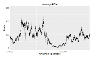
The test:  To test whether the new strategy works, the PhD student first created a set of four fake-uptake samples by adding 10% of Rd reads (set 1) to each of the four input samples (NP-long, NP-short, GG-long, GG-short).  He then created the corresponding fake-contaminated input samples by adding different Rd reads (set 2) to get the same 10% contamination level.  He then calculated and plotted the ratio of fake-uptake to fake-input for each genome position.  If the contamination correction were perfect this would give a value of 1.0 at every position, but we knew it would be imperfect because the contamination reads (set 1) and the correction reads (set 2) were not identical.

Here are the results for the NP-long analysis (the NP-short was similar):

The top graph shows a 10 kb segment; the bottom one the whole genome.  The uptake rations are nicely centered at 1.0, varying from about 0.9 to about 1.1.  This variation is expected, due to the random differences in Rd coverage by set 1 and set 2.  The segments with no variation are places where the Rd genome has no homolog in the NP sequences.

Here are results for GG-long:

This result is noisier, with many spikes above 1.1 and dips below 0.9.  The cause was easy to find:  the spikes and dips occur at positions where sequencing inefficiencies cause very low GG coverage.  Below are coverage graphs for the 10 kb segment in the first graph above, and for a 30 kb segment around the major spike/dip at position 400,000 in the whole-genome graph above.  In each case we see that sequencing coverage is much lower at the spike-dip positions, causing the chance differences in Rd coverage to have a much bigger effect than elsewhere. 

In principle, the role of chance differences between the set 1 and set 2 Rd coverage can be checked by examining the other GG sample, GG-short, but I think the PhD student used exactly the same sets of Rd reads for this sample as for the others, which would predict that the spikes and dips should be the same.  They're not, probably because of differences in GG coverage between the long and short samples.

We should go back and test the same GG-long sample using different sets of Rd reads (set 3 rather than set 1, or set 4 rather than set 2).

Sources of variation:  The above analysis gives us a better understanding of the sources of variation in this uptake analysis.  First there's the variation across the genome in sequencing efficiency.  This is (we think) due to properties of the sequencing technology, and should be constant across different samples from the same genome (e.g. input and uptake samples). We don't have any way to reduce this variation, but we control for it by calculating the uptake ratios rather than just position-specific differences in coverage in the uptake samples.  Second, there's the variation in how much Rd contamination is present.  This arises due to variation in the experiments that purified the DNA; we can't change it at this stage, but we control for the differences between samples by introducing different amounts of compensating fake-contamination into the input sample control for each uptake sample.  Third, there's the chance variation in the distribution of contaminating Rd reads across the genome.  This will be different for each sample, and we can't change it or control for it.  Finally there's the random variation in the distribution of fake-contaminating Rd reads added to each input sample.  The next section describes how we can eliminate most of this.

Replicate corrections will reduce variation:  The above analysis also showed us a way to improve the correction in our 12 genuinely contaminated samples.  Instead of doing each correction once, we can do the correction several times, generating independent fake-contamination input samples using independent sets of Rd reads.  Then we can average the resulting uptake ratios.  In fact we can do this a simpler way, by just averaging the coverage levels of the independent fake-contamination input samples at each position, and then calculating the uptake ratios using these averages.

The number of Rd reads needed for each correction will depend on the coverage level and true contamination level of each uptake sample, but we should have enough Rd reads to create at least five four independent sets for each sample (see next post).